XGBoost Model Tutorial

Welcome! In this guide, you'll learn how to train a Gradient Boosting Classifier based on the XGBoost library in a federated manner using the Apheris platform.

We'll explore how this powerful decision-tree-based machine learning model can predict patient outcomes from medical data collected at multiple locations without moving the data.

Why XGBoost?

XGBoost (Extreme Gradient Boosting) is a powerful, scalable machine learning library ideal for structured data analysis, renowned for its predictive performance and speed. It builds ensembles of decision trees, effectively capturing complex data patterns. Using NVIDIA FLARE's XGBoost components, Apheris allows secure federated training on distributed data sources.

Installation

First, please follow Quickstart: Installing the Apheris CLI to ensure you have the CLI and its dependencies installed.

The Apheris XGBoost model can take FederatedDataFrames as input.

Therefore, please also install the Apheris Statistics wheel, as described in Simulating and Running Statistics Workflows.

Finally, install the Apheris XGBoost wheel as below (replace x.y.z with the version number of your wheel file):

pip install apheris_xgboost-x.y.z-py3-none-any.whl

Now login to Apheris using the Python API:

import apheris

apheris.login()

To visualize the models you'll train later in this guide, you also need to first install graphviz binaries onto your machine, then install the graphviz Python package into your virtual environment.

pip install graphviz

Understanding Compute Specs

A Compute Spec is a crucial element in Apheris, defining how computational tasks are securely executed on datasets owned by Data Custodians. For detailed understanding, see Compute Specs documentation.

First, create a Compute Spec using the Apheris Python API (see here for more information):

from aphcli.api import compute

compute_spec_id = compute.create_from_args(
    dataset_ids=["whas1_gateway-1_org-1","whas2_gateway-2_org-2"],
    model_id='apheris-xgboost',
    model_version="0.14.0",
    client_memory=1024,
    client_n_cpu=1,
    client_n_gpu=0,
    server_memory=1024,
    server_n_cpu=1,
    server_n_gpu=0,
)

Note

Here we are only training a simple classifier, which is relatively shallow and only has a small number of parallel trees. If you are building a more complex model, you may need to increase the compute resources shown above.

Once you've created your Compute Spec, you have to activate it in order to start the computation. Once activated, you can run multiple jobs against the same Compute Spec, until it is deactivated.

compute.activate(compute_spec_id)

Depending on the computational requirements, it may take a minute or two for your Compute Spec to activate.

You can check the status of your Compute Spec like so:

compute.get_status(compute_spec_id)

The following command will wait until the Compute Spec is activated, then return:

compute.wait_until_running(compute_spec_id)

The XGBoostSession

The XGBoostSession objects - specifically XGBoostLocalSession and XGBoostRemoteSession - are used for managing the federated training context. They abstract the complexity involved in federated learning sessions, managing data access, security boundaries, and computation context.

Local Session (XGBoostLocalSession)

This session type is designed primarily for development, experimentation, and debugging purposes. It simulates a federated environment locally, meaning it:

• Operates on datasets stored on your local filesystem.
• Requires explicit mappings of simulated Gateway IDs to local dataset paths.
• Helps you validate your workflows before remote execution.

Important

In order to support Federated Learning in a local environment, you must be on the Linux operating system, or compile XGBoost from source, as there is no pre-compiled wheel available for other operating systems with Federated Learning support. Running with an incompatible wheel will result in the following error: XGBoost is not compiled with federated learning support.

from pathlib import Path
from apheris_xgboost.session import XGBoostLocalSession

# insert your local file path here
local_path = f"{Path.home()}/data"
filenames_per_client = {
    "site-1": ["whas1-data.csv"],
    "site-2": ["whas2-data.csv"],
}
local_session = XGBoostLocalSession(
    dataset_root=local_path,
    dataset_mapping=filenames_per_client, 
    workspace="/tmp/xgboost",
)

Parameters:

• dataset_root: Root directory containing the local datasets.
• dataset_mapping: Maps simulated Gateway IDs to filenames of the datasets (relative to dataset_root).
• workspace: Local path where intermediate and output data are stored.

Remote Session (XGBoostRemoteSession)

This session type facilitates actual federated training on remote Gateways. It uses the ID of the Compute Spec you created earlier and dispatches jobs to the Gateways via a simple Python interface.

from apheris_xgboost.session import XGBoostRemoteSession

remote_session = XGBoostRemoteSession(
    compute_spec_id=compute_spec_id,
    dataset_ids=["whas1_gateway-1_org-1", "whas2_gateway-2_org-2"]
)

Parameters:

• compute_spec_id: Unique identifier of an existing, activated Compute Spec.
• dataset_ids: Identifiers of the datasets residing on remote Gateways for federated analysis.

Train your model

You're about to train a model to predict patient survival (fstat) using selected patient attributes:

• afb: Atrial Fibrillation
• age: Patient's age
• bmi: Body Mass Index
• chf: Congestive Heart Complications

To start the training use the Apheris function fit_xgboost. You can choose whether to run locally or on the remote Gateways by providing the relevant session.

Now run a remote training job on Apheris Gateways:

from apheris_xgboost.api_client import fit_xgboost

target_col = "fstat"
cols = ["afb", "age", "bmi", "chf"]

model = fit_xgboost(
    num_rounds=10,
    target_col=target_col,
    cols=cols,
    eta=0.2,
    eval_metric="mae",
    max_depth=3,
    num_parallel_tree=5,
    session=remote_session,
)

Note

For the remainder of this guide, we'll train on remote Gateways. To train on local session, simply change remote_session for the local_session described above.

Training arguments

Apheris-specific parameters:

• session: The session object used for managing the training process within the Apheris platform.
• target_col: The target column in the dataset that the model aims to predict.
• cols: The list of feature columns used for training the model.
• datasets: An optional list of FederatedDataFrames representing the datasets to fit the model to. If not provided, the session's dataset mapping will be used without any preprocessing.
• timeout: The timeout setting for the NVIDIA FLARE task. For remote training jobs, this is also used as the Apheris job timeout with an additional buffer of 60 seconds.

XGBoost parameters:

• num_rounds: Specifies the number of boosting iterations. In XGBoost, this is often referred to as num_boost_round.
• eta: The learning rate, which scales the contribution of each tree. It helps prevent overfitting by shrinking the weights.
• max_depth: Determines the maximum depth of the trees. Increasing this value makes the model more complex and more likely to overfit.
• num_class: Specifies the number of classes for multi-class classification. Used when objective is set to a multi-class classification loss.
• objective: Defines the learning task and the corresponding loss function, such as reg:squarederror for regression tasks.
• eval_metric: Specifies the evaluation metrics to be monitored during training. For example, rmse for root mean square error.
• num_parallel_tree: Used for boosting random forests. It specifies the number of trees to grow in parallel in each round.
• enable_categorical: Indicates whether to treat certain features as categorical. When set to true, XGBoost will handle categorical features directly.
• feature_types: A list indicating each feature's data type ('float', 'int', 'categorical') when categorical feature handling is enabled
• tree_method: Specifies the tree construction algorithm used in XGBoost. Options include auto, exact, approx, hist, and gpu_hist.
• early_stopping_rounds: Activates early stopping. Training stops if the evaluation metric doesn't improve for a given number of rounds.
• nthread: Specifies the number of parallel threads used to run XGBoost.

Important

If you are running training on a larger dataset, you may find the default timeout is insufficient. In this case, you can increase it to suit your needs using the timeout parameter.

Examining your model

The model object returned by fit_xgboost is a serialized representation of the trained model, which is directly compatible with XGBoost. Yours should look something like this:

    {'learner': {'attributes': {'best_iteration': '1',
       'best_score': '0.3502602116332028'},
      'feature_names': ['afb', 'age', 'bmi', 'chf'],
      'feature_types': ['float', 'float', 'float', 'float'],
      'gradient_booster': {'model': {'gbtree_model_param': {'num_parallel_tree': '5',
         'num_trees': '5'},
        'iteration_indptr': [0, 5],
        'tree_info': [0,
         0,
         0,
         0,
         0,],
        'trees': [{'base_weights': [
            6.802704e-09,
            -0.09351389,
            ...
           0.0054957066],
          'categories': [],
          'categories_nodes': [],
          'categories_segments': [],
          'categories_sizes': [],
          'default_left': [0, 0, 0, 0, 0, 0, 0, 0, 0, 0, 0, 0, 0, 0, 0],
          'id': 0,
          'left_children': [1, 3, 5, 7, 9, 11, 13, -1, -1, -1, -1, -1, -1, -1, -1],
          'loss_changes': [ 2.6578097, 1.9690572, ... 0.0],
          'parents': ...,
          'right_children': ...,
          'split_conditions': ...,
          'split_indices': ...,
          'split_type': ...,
          'sum_hessian': ...,
          'tree_param': {'num_deleted': '0',
           'num_feature': '4',
           'num_nodes': '15',
           'size_leaf_vector': '1'}},
        ...
      ]},
       'name': 'gbtree'},
      'learner_model_param': {'base_score': '6.557377E-1',
       'boost_from_average': '1',
       'num_class': '0',
       'num_feature': '4',
       'num_target': '1'},
      'objective': {'name': 'reg:squarederror',
       'reg_loss_param': {'scale_pos_weight': '1'}}},
     'version': [2, 1, 1]}

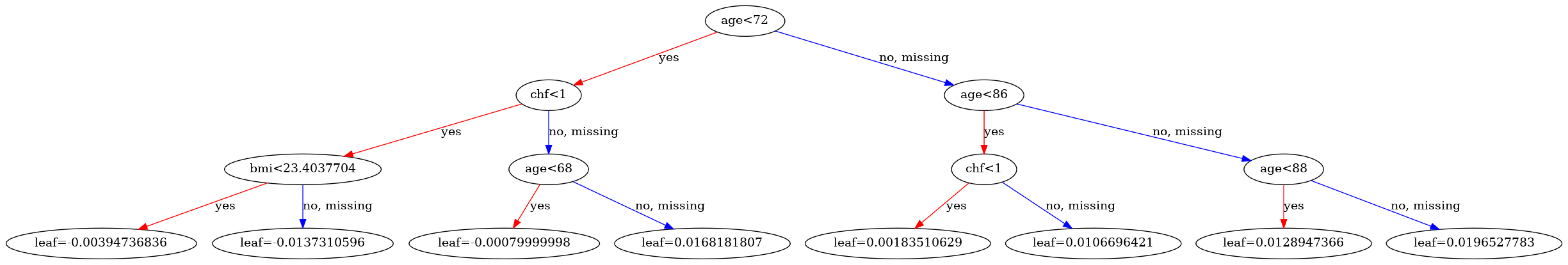
Since the model is compatible with XGBoost, you can visualize the trees using XGBoost's visualization functions:

import json
from tempfile import TemporaryDirectory

from xgboost import plot_tree
from xgboost.core import Booster
from matplotlib.pylab import rcParams

def model_to_booster(model: dict) -> Booster:
    with TemporaryDirectory() as tmp_model_dir:
        model_file = tmp_model_dir / "model.json"
        model_file.write_text(json.dumps(model))
        booster = Booster()
        booster.load_model(str(model_file))
    return booster


def visualize_model(model, num_tree):
    booster = model_to_booster(model)
    rcParams['figure.figsize'] = 80, 50
    plot_tree(booster, num_trees=num_tree)

visualize_model(model, num_tree=1)

Note

If you are using the macOS operating system, you may receive an import error: XGBoostError: XGBoost Library (libxgboost.dylib) could not be loaded. To resolve this, install libomp onto your machine using, e.g. Homebrew: brew install libomp.

You can alternatively view the model as a dataframe, again using XGBoost's own APIs:

import pandas as pd

def convert_model(model: dict)-> pd.DataFrame:
    booster = model_to_booster(model)
    return booster.trees_to_dataframe()

convert_model(model)

	Tree	Node	ID	Feature	Split	Yes	No	Missing	Gain	Cover	Category
0	0	0	0-0	age	72.00000	0-1	0-2	0-2	19.258240	384.0	NaN
1	0	1	0-1	chf	1.00000	0-3	0-4	0-4	5.252416	183.0	NaN
2	0	2	0-2	age	86.00000	0-5	0-6	0-6	3.807554	201.0	NaN
3	0	3	0-3	bmi	23.40377	0-7	0-8	0-8	0.895349	149.0	NaN
4	0	4	0-4	age	68.00000	0-9	0-10	0-10	1.468441	34.0	NaN
...	...	...	...	...	...	...	...	...	...	...	...
75	4	10	4-10	Leaf	NaN	NaN	NaN	NaN	-0.010831	2.0	NaN
76	4	11	4-11	Leaf	NaN	NaN	NaN	NaN	0.001604	120.0	NaN
77	4	12	4-12	Leaf	NaN	NaN	NaN	NaN	-0.000931	205.0	NaN
78	4	13	4-13	Leaf	NaN	NaN	NaN	NaN	0.003282	25.0	NaN
79	4	14	4-14	Leaf	NaN	NaN	NaN	NaN	0.007388	10.0	NaN

Debugging Gateway Errors

When something goes wrong, the fit_xgboost function will raise a RuntimeError, the message for which contains the logs from the Apheris Orchestrator.

You can use these logs to diagnose the issue.

To illustrate this, attempt to run a training job with an invalid input column name:

cols_with_typo = [
"afb", "age", "bmi", "chff"
]

try:

    model = fit_xgboost(
        num_rounds=10,
        target_col=target_col,
        cols=cols_with_typo,
        eta=0.2,
        eval_metric="mae",
        max_depth=3,
        num_parallel_tree=5,
        session=remote_session,
    )

except RuntimeError as e:
    error_logs = str(e)

Now, to find the source of the error; split the logs to lines and find all error lines:

error_rows = [l for l in error_logs.split("\n") if "ERROR" in l]
print(error_rows[0])

"2025-03-11 18:41:33,229 - ClientLogForwarder - ERROR - [identity=Unnamed_project_69bc2e32-001e-4cd5-95c5-a219a674590a, run=5a419738-3c20-4bba-aae6-186bc9f1fc61, wf=xgb_controller]: ClientLogForwarder: Message from 'b312cc05-da9d-70c2-d8c9-51af2f9f726a [ERROR]': Exception of type 'ValueError' has occurred in /workspace/src/apheris_xgboost/data_loader.py:153 (function: 'load_data')."

Let's look a bit more closely at this...

• Timestamp (2025-03-11 18:41:33,229):
  The exact date and time (UTC) when the error occurred.

• Component (ClientLogForwarder):
  Indicates which internal component logged the error. In this case, ClientLogForwarder is responsible for sending logs from client Gateways back to the central Orchestrator. You cannot see logs from the Gateways themselves, since that could reveal sensitive information.

• Exception Type (ValueError): Identifies the kind of exception raised, giving an immediate indication of what went wrong. Here, ValueError suggests an issue with input values or data formats.

• Source (data_loader.py:153, function: load_data): Clearly pinpoints the exact source code file, line number, and function where the error was raised, making it easier to debug.

Using this structured breakdown, you can quickly locate, diagnose, and resolve errors within your federated training workflows.

Advanced Usage - Pre-processing with FederatedDataFrame

The datasets parameter of fit_xgboost can be None, in which case training occurs on all datasets in the Compute Spec, or it can take a list of dataset IDs to specify which datasets to use in the model training. In both cases, the model is trained on the raw data held in those datasets.

However, it is often helpful to perform a some pre-processing on the input data before passing using it to train a model. To enable this, the dataset parameter also accepts a list of FederatedDataFrames instead of the dataset IDs.

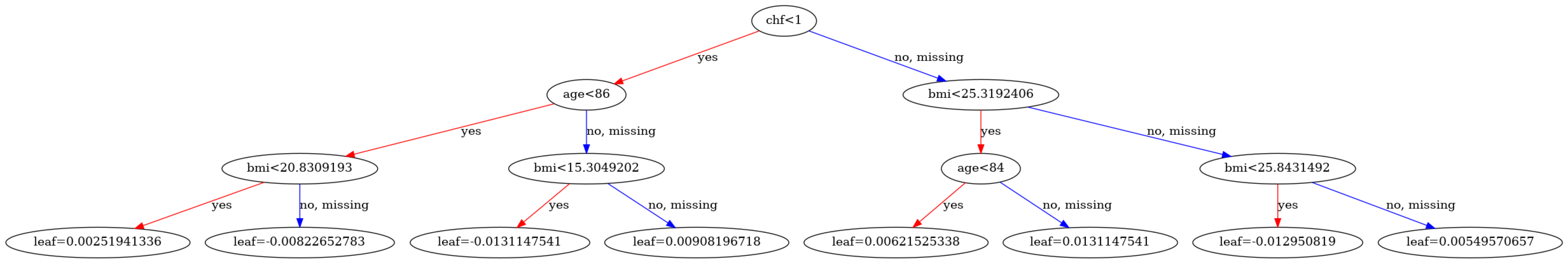
A FederatedDataFrame always refers to a dataset ID. Once the FederatedDataFrames are created, you can proceed with the preprocessing as usual. In the following, you'll use the FederatedDataFrame to filter the data to patients with age larger than 72.

from apheris_stats.simple_stats.util import FederatedDataFrame

fdf1 = FederatedDataFrame("whas1_gateway-1_org-1")
fdf2 = FederatedDataFrame("whas2_gateway-2_org-2")

fdf1 = fdf1[fdf1["age"] > 72]
fdf2 = fdf2[fdf2["age"] > 72]
datasets = [fdf1, fdf2]

cols = [
"afb", "age", "bmi", "chf"
]

model = fit_xgboost(
    datasets=datasets,
    num_rounds=10,
    target_col=target_col,
    cols=cols,
    eta=0.2,
    eval_metric="mae",
    max_depth=3,
    num_parallel_tree=5,
    session=remote_session,
)

Comparing the first trees of the model trained on filtered data, you can see that the age decision bounds reflect the new distribution.

visualize_model(model, num_tree=1)

Using FederatedDataFrames locally

You can also use the FederatedDataFrame in local sessions, you just have to ensure that the dataset IDs used in the FederatedDataFrame match those used in the ds2gw_dict parameter passed to the XGBoostLocalSession:

Note that you don't need to redefine the FederatedDataFrames that you used above as the dataset IDs in ds2gw_dict match the ones used in the remote run. The session simply uses them to find the local data - the actual file paths come from the filenames_per_client dictionary you created at the start of this guide.

Apheris XGBoost supports all the objectives available in vanilla XGBoost. For a full list, see the XGBoost documentation. We want to train a model to estimate the binary value fstat, use the binary:logistic objective to get a probability of fstat=1.

local_session = XGBoostLocalSession(
    dataset_mapping=filenames_per_client,
    ds2gw_dict = {'whas1_gateway-1_org-1': 'site-1', 'whas2_gateway-2_org-2': 'site-2'},
    workspace="/tmp/xgboost",
    dataset_root=local_path
)

model = fit_xgboost(
    datasets=datasets,
    num_rounds=10,
    target_col=target_col,
    cols=cols,
    eta=0.2,
    objective="binary:logistic",
    eval_metric="mae",
    max_depth=3,
    num_parallel_tree=5,
    session=local_session,
)

Evaluating your new model

To ensure the model trained above is useable, it should be evaluated against a holdout dataset.

In this case, for simplicity, we'll just the training set, but in a realistic setting you'd ensure there was a separate dataset available for evaluation.

from apheris_xgboost.api_client import evaluate_xgboost

eval_results = evaluate_xgboost(
    model_parameter=model,
    target_col=target_col,
    feature_cols=cols,
    objective="binary:logistic",
    session=remote_session,
)

Evaluation arguments

Apheris-specific parameters:

• session: The session object used for managing the training process within the Apheris platform.
• model_parameter: A dictionary containing model parameters for initializing the prediction model.
• target_col: The target column in the dataset that the model aims to predict.
• feature_cols: The list of feature columns used for predictions.
• datasets: An optional list of FederatedDataFrames representing the datasets to fit the model to. If not provided, the session's dataset mapping will be used without any preprocessing.
• additional_eval_metric: Additional evaluation metrics from scikit-learn; can only be specified when using the multi:softmax objective.
• timeout: The timeout setting for the NVIDIA FLARE task. For remote training jobs, this is also used as the Apheris job timeout with an additional buffer of 60 seconds.

XGBoost parameters:

• eval_metric: Metric(s) used by XGBoost to evaluate model performance (e.g., "rmse", "logloss", "auc").
• num_class: Specifies the number of classes for multi-class classification. Used when objective is set to a multi-class classification loss.
• objective: Defines the learning task and the corresponding loss function, such as reg:squarederror for regression tasks.
• quantile_alpha: The quantile level (alpha) required when using the reg:quantileerror objective for quantile regression.

Output format

The resulting dictionary gives you the evaluation score for each dataset. The dictionary keys are the Gateway IDs that refer to the datasets, and the values are lists, where each element is the prediction result for each row of the prediction dataset. You can use the message printed to map the Gateway ID back to the dataset ID.

Running XGBoost prediction job on {'b312cc05-da9d-70c2-d8c9-51af2f9f726a': ['whas/worcester/data.csv'], 'a6600818-fd6f-e994-2f7a-f687710d2021': ['whas/norfolk/data.csv']}
You provided the job ID ae362ba6-7d9f-4b98-818b-6d51dc03896c.
You provided the job ID ae362ba6-7d9f-4b98-818b-6d51dc03896c.

{'b312cc05-da9d-70c2-d8c9-51af2f9f726a': ['eval-logloss:0.64586037009954456'],
 'a6600818-fd6f-e994-2f7a-f687710d2021': ['eval-logloss:0.61601662024071346']}

Using your new model for prediction

Now you've trained your model, you can use it to predict outcomes.

In this example, you'll retrieve these for the training set, but in a realistic scenario you would likely create and use a new Compute Spec with access to the dataset to be predicted.

from apheris_xgboost.api_client import predict_xgboost

probabilities_by_gateway = predict_xgboost(
    model_parameter=model,
    feature_cols=cols,
    objective="binary:hinge",
    num_class=2,
    session=remote_session,
)

Prediction arguments

Apheris-specific parameters:

• session: The session object used for managing the training process within the Apheris platform.
• model_parameter: A dictionary containing model parameters for initializing the prediction model. This is what is returned by fit_xgboost.
• target_col: The target column in the dataset that the model aims to predict.
• feature_cols: The list of feature columns used for predictions.
• datasets: An optional list of FederatedDataFrames representing the datasets to fit the model to. If not provided, the session's dataset mapping will be used without any preprocessing.
• timeout: The timeout setting for the NVFlare task. For remote training jobs, this is also used as the Apheris job timeout with an additional buffer of 60 seconds.

XGBoost parameters:

• num_class: Specifies the number of classes for multi-class classification. Used when objective is set to a multi-class classification loss.
• objective: Defines the learning task and the corresponding loss function, such as reg:squarederror for regression tasks.
• quantile_alpha: The quantile level (alpha) required when using the reg:quantileerror objective for quantile regression.

Output format

The resulting dictionary gives you the probabilities for each sample in the dataset. The dictionary keys are the Gateway IDs that refer to the datasets, and the values are lists, where each element is the prediction result for each row of the prediction dataset. You can use the message printed to map this back to the dataset ID.

Running XGBoost prediction job on {'b312cc05-da9d-70c2-d8c9-51af2f9f726a': ['whas/worcester/data.csv'], 'a6600818-fd6f-e994-2f7a-f687710d2021': ['whas/norfolk/data.csv']}
You provided the job ID fafe196e-7f46-442e-a28d-f6204d10366e.
You provided the job ID fafe196e-7f46-442e-a28d-f6204d10366e.

{'b312cc05-da9d-70c2-d8c9-51af2f9f726a': [0.47880467772483826,
  0.13351966440677643,
  0.36020007729530334,
  0.635794460773468,
  ...],
  'a6600818-fd6f-e994-2f7a-f687710d2021': [...]}

Deactivate your Compute Spec

Now you're all done, it is important to deactivate your Compute Spec to avoid incurring unexpected costs:

compute.deactivate(compute_spec_id)

Summary

In this tutorial, you have been introduced to the Apheris XGBoost model, and learned how to train some basic tree-based models.

If you'd like to learn more about how to interact with the Apheris environment, we'd recommend the Getting started with Apheris CLI guide, or to find out more about how to use the Statistics package to analyse data in a secure and privacy-preserving way, check out our guide to Simulating and Running Statistics.