Common Statistics Functions

This guide will walk you through some of the commonly used functions and workflows in Apheris Statistics. It assumes you've already worked through Simulating and Running Statistics Workflows, and are familiar with the basic workflow. If you haven't already, please work through that tutorial before starting this one.

First, import apheris and login to the environment:

import apheris
from aphcli.api import datasets
from apheris_stats.simple_stats.util import FederatedDataFrame, SimpleStatsSession, provision
from apheris_stats import simple_stats

apheris.login()

Logging in to your company account...
Apheris:
Authenticating with Apheris Cloud Platform...
Please continue the authorization process in your browser.
Gateway:
Authenticating with Apheris Compute environments...
Please continue the authorization process in your browser.

Take another look at the datasets, which are available to you:

datasets.list_datasets()

Output:

+-----+-------------------------+--------------+---------------------+
| idx |         dataset_id      | organization |   data custodian    |
+-----+-------------------------+--------------+---------------------+
|  0  |  whas2_gateway-2_org-2  |    Org 2     |     Orsino Hoek     |
|  1  |  whas1_gateway-1_org-1  |    Org 1     |  Agathe McFarland   |
| ... |          ...            |     ...      |         ...         |
+-----+-------------------------+--------------+---------------------+

In this tutorial you will again work on the datasets whas1_gateway-1_org-1 and whas2_gateway-2_org-2.

As a reminder, these are synthetically generated datasets that contain medical data. Both are CSV files and have same structure. One resides on the Gateway of Organization "Org 1" and the other is with "Org 2".

simple_stats_session = provision(
    dataset_ids=[
        "whas1_gateway-1_org-1", "whas2_gateway-2_org-2"
    ]
)

simple_stats_session

compute_spec_id: 7b6d7e19-a364-4c2e-85d1-2038d4a00101

Successfully activated ComputeSpec!

SimpleStatsSession(compute_spec_id='7b6d7e19-a364-4c2e-85d1-2038d4a00101')

The provisioning returns a SimpleStatsSession object. The compute_spec_id is an ID that refers to the cluster that has just been activated.

If you wanted to reuse an existing activated compute spec with a new Apheris statistics script, you can instantiate a new session with it:

my_compute_spec_id = simple_stats_session.compute_spec_id
my_second_session = SimpleStatsSession(my_compute_spec_id)
my_second_session

SimpleStatsSession(compute_spec_id='7b6d7e19-a364-4c2e-85d1-2038d4a00101')

Now, create a FederatedDataFrame on the first dataset; whas1_gateway-1_org-1 and another for the second; whas2_gateway-2_org-2:

dataset_ids = ["whas1_gateway-1_org-1", "whas2_gateway-2_org-2"]

fdf_whas1 = FederatedDataFrame(dataset_ids[0])
fdf_whas2 = FederatedDataFrame(dataset_ids[1])

You can investigate the structure of a dataset using the describe function. This will tell you some meta information about the dataset, but without revealing the actual source data.

Run describe on the FederatedDataFrame for the whas1_gateway-1_org-1 dataset to see what columns are available and some basic statistics:

description = simple_stats.describe(fdf_whas1, simple_stats_session)

description[dataset_ids[0]]["results"]

	type	count	count_nan	num_unique_values	percentile_5th	percentile_95th
afb	float64	100	0	2	0	1
age	float64	100	0	45	48	89
av3	float64	100	0	2	0	0
bmi	float64	100	0	95	18.6	35.3
chf	float64	100	0	2	0	1
cvd	float64	100	0	2	0	1
diasbp	float64	100	0	54	49	116.2
gender	float64	100	0	2	0	1
hr	float64	100	0	60	49.8	133.1
los	float64	100	0	19	2	16
miord	float64	100	0	2	0	1
mitype	float64	100	0	2	0	1
sho	float64	100	0	2	0	1
sysbp	float64	100	0	64	97	200.3
fstat	bool	100	0	2	NaN	NaN
lenfol	float64	100	0	91	3	2175.2

Running statistical operations

The first statistics function you'll use here is the count_null function, which counts the number of null values in a column of a dataset. In this example, you will provide one of the FederatedDataFrames from above to run on that dataset:

result = simple_stats.count_null(
    fdf_whas1,
    column_name="age",
    aggregation=True,
    session=simple_stats_session
)

result

		count_null
total	NA values	0
not NA values	100

This time, do the same, but pass both the FederatedDataFrames from above. This means your operation will run on multiple Compute Gateways at the same time.

You'll see aggregation=True is set; which means that the results from each Compute Gateway will be aggregated prior to returning them to you.

result = simple_stats.count_null(
    [fdf_whas1, fdf_whas2],
    column_name="age",
    aggregation=True,
    session=simple_stats_session
)

result

		count_null
total	NA values	0
not NA values	480

Now switch aggregation off to see the per dataset results:

result = simple_stats.count_null(
    [fdf_whas1, fdf_whas2],
    column_name="age",
    aggregation=False,
    session=simple_stats_session
)

result

{'whas1_gateway-1_org-1': {'results':                          count_null  count
  total age NA values               0    100
            not NA values         100    100},
 'whas2_gateway-2_org-2': {'results':                          count_null  count
  total age NA values               0    380
            not NA values         380    380}}

You can see a full list of statistics functions in the Statistics Reference. You'll see many of the functions are used in a similar way; for example we can use mean_column instead of count_null to calcualte the mean age over the data:

result = simple_stats.mean_column(
    [fdf_whas1, fdf_whas2],
    column_name="age",
    aggregation=True,
    session=simple_stats_session
)

result

69.58333333333334

You can group results by other columns to get more insight into the data. Here we'll use gender, which is categorised numerically as 0 or 1 in this dataset:

result = simple_stats.mean_column(
    [fdf_whas1, fdf_whas2],
    column_name="age",
    group_by="gender",
    aggregation=True,
    session=simple_stats_session
)

result

	mean_column
0.0	66.193772
1.0	74.712042
total	69.583333

Advanced example: Summary statistics

This, more advance example will demonstrate how to use the pre-processing functionality in the FederatedDataFrame to manipulate the input data in preparation for analysis. You'll then use the tableone function to capture a number of summary statistics about the data.

def prepare_dates(federated_df):
    for col in ["sysbp"]:
        federated_df.loc[:,col] = federated_df.loc[:,col].to_datetime(unit='M')

    for col in ["fstat", "gender", "age"]:
        federated_df.loc[:,col] = federated_df.loc[:,col].astype("int")

    federated_df["sysbpyr"] = federated_df["sysbp"].dt.year
    return federated_df

all_datasets = [fdf_whas1, fdf_whas2]

prepped_datasets = [prepare_dates(d) for d in all_datasets]

numerical_columns = ["hr", "los", "sysbpyr", "fstat", "gender"]

table_one_result = simple_stats.tableone(
    session=simple_stats_session,
    datasets=prepped_datasets,
    numerical_columns=numerical_columns, 
    numerical_nonnormal_columns=numerical_columns
)

table_one_result

	col	category	n	mean	std	min	quartile_1	median	quartile_3	max
0	fstat	total	480	0.422917	0.494022	0.0	0.01	0.01	0.99	1.0
1	los	total	480	6.185417	4.767183	0.0	2.82	4.70	7.99	47.0
2	sysbpyr	total	480	1981.495833	2.681725	1974.0	1979.92	1980.88	1982.96	1990.0
3	hr	total	480	86.660417	23.661134	35.0	68.22	84.83	99.93	186.0
4	gender	total	480	0.397917	0.489468	0.0	0.01	0.01	0.99	1.0

Advanced example: Kaplan Meier statistics

In this final example, you will use Kaplan-Meier to estimate a survival function, measuring the likelihood of the occurrence of a certain event over time.

This example uses a combination of FederatedDataFrame pre-processing and the kaplan_meier function from Apheris Statistics to calculate the likelihood of survival of a patient with respect to some event fstat.

kaplan_meier_result = simple_stats.kaplan_meier(
    session=simple_stats_session,
    datasets=prepped_datasets,
    duration_column_name="age",
    event_column_name= "fstat",
    stepsize=1,
    plot = True
)

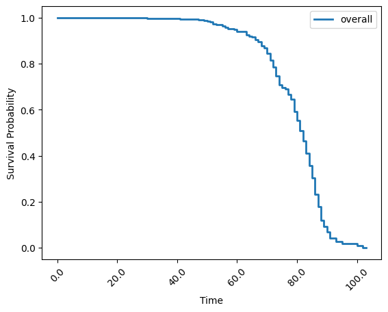
The plot that was created by simple_stats.kaplan_meier gives us a first simple visualization. As you have the raw data kaplan_meier_result, you could use your own plotting tools to generate similar figures.

kaplan_meier_result

{'overall':                       survival_function  cumulative_distribution
 total (-0.001, 1.0]            1.000000                 0.000000
       (1.0, 2.0]               1.000000                 0.000000
       (2.0, 3.0]               1.000000                 0.000000
       (3.0, 4.0]               1.000000                 0.000000
       (4.0, 5.0]               1.000000                 0.000000
 ...                                 ...                      ...
       (99.0, 100.0]            0.017072                 0.982928
       (100.0, 101.0]           0.017072                 0.982928
       (101.0, 102.0]           0.008536                 0.991464
       (102.0, 103.0]           0.008536                 0.991464
       (103.0, 104.0]           0.000000                 1.000000

 [104 rows x 2 columns]}

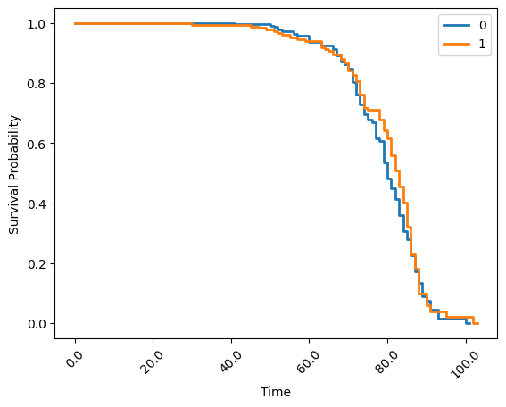
Finally, you can use groupings on kaplan_meier to visualise data by some category. In this case, use the gender column to group the analysis above:

kaplan_meier_result = simple_stats.kaplan_meier(
    session=simple_stats_session,
    datasets=prepped_datasets,
    duration_column_name="age",
    event_column_name= "fstat",
    group_by="gender",
    stepsize=1,
    plot = True
)

Close the session

When we are finished, we close the session. This deactivates the deployed cluster, freeing up resources and reducing infrastructure costs.

simple_stats_session.close()

Summary

In this tutorial, you have walked through some of the key statistics functions available to you and see how to use groupings to further explore the data. You have experimented with tableone analysis and visualised survival statistics using Kaplan-Meier.

For more information on the functions you can use with Apheris Statistics, see the Statistics Reference document