Apheris Regression Models🔗
The apheris-regression-models package contains the following regression models:
- Logistic Regression Model
- Cox Proportional Hazard Model
Both are Federated implementations that run on Apheris. All regression models are implemented as NVIDIA FLARE projects and follow the same code structure:
- Learner: extends a common superclass
RegressionLearner - Client API: contains the python interface to call the training flow. It expects a
SupervisedMLSessionas well as the model and training parameters and submits the job.
Logistic Regression🔗
The Logistic Regression Model describes the probability that the dependent variable Y is equal to 1 given a set of independent variables X.
The parameters of the model are the regression coefficients. The intercept \(a\) can be written as \(a= \exp(-\beta_0)\). Equation (1) is a sigmoid function. The Logistic Regression Model is equivalent to a shallow neural network with one linear layer and sigmoid activation.
Linear Regression🔗
Linear regression fits a vector of regression coefficients to a given feature dataset. For more information see
LinearRegression.
Federated Implementation🔗
The implementation of the Logistic regression model is based on scikit-learn.
The model parameters \(\beta\) and \(a\) are trained on each local dataset and aggregated with Federated Averaging on a central orchestrator.
Feature Selector🔗
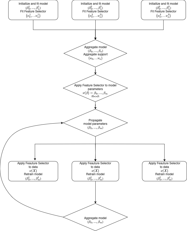
The Logistic Regression Model can be used in combination with a feature selector. Currently it is implemented with scikit-learn's SequentialFeatureSelector. The features are selected separately on each client and aggregated by majority vote. That means each client is weighted by the number of its data points and contributes a value 0 or 1, indicating if this feature is to be selected or not. If the weighted average over all clients is greater than 0.5 the feature will be selected; otherwise, it will not. The feature selection takes place at initialization time of the learner and is trained on each dataset. However, in Federated Training, we have to ensure that all clients are performing the local training on the same set of features. Otherwise, the parameters cannot be aggregated afterward. To see this, we consider the following example:
Client 1 and 2 have training datasets containing features A,B,C and D. Now we apply feature selection in the initial round. Let's assume that:
- Client 1 selects features A and B,
- Client 2 selects features B, C and D.
If the local training now takes only the selected features into account, we end up with model parameters (i.e. the regression coefficients) that can not be aggregated as they refer to different features.
To solve this we train the logistic regression model in the first round on the full feature set. The support vector of the feature selector is aligned over the clients by majority vote. This happens only in the first aggregation round and once this is done, the regression coefficients model parameter is transformed in the same way as the training data. From the second round on the local training rounds are only trained on the selected features and the feature selector remains frozen. The training flow with feature selection is illustrated in the figure below.
Python API🔗
To fit the Logistic Regression model via the Python API use the following method:
result = fit_lr(
        datasets=datasets,
        session=session,
        feature_cols=[
            "column_1",
            "column_2",
            "column_3",
            "column_4"
        ],
        target_col="event",
        validation_set_col="val",
        feature_selector_direction="backward",
        num_rounds=3,
        num_steps_per_round = 10,
        model_type = "logistic_regression",
)
To fit a LinearRegression model use model_type=linear_regression.
The parameter feature_selector_direction determines the feature selection mode. It defaults to None. In this case, no feature selection is applied.
Cox Proportional Hazard Model🔗
Cox proportional hazard model is consisting of a baseline hazard \(\lambda_0(t)\) and a partial hazard \(\exp(\beta x)\) for individual x to have an event at time \(t\).
The parameter estimation of the Cox model is carried out by maximizing the log-likelihood function:
where \(R(x_i)\) denotes the risk set for the event time of \(x_i\). That means it contains all individuals \(x_j\) that are still at risk after the time point of the hazard event for individual \(x_i\).
Federation🔗
We can see that this likelihood is not separable as it depends on the full risk set even if the individuals are separated over several clusters. In our Cox implementation we follow [2] and optimize instead a stratified approximation of this likelihood, stratified over the different clusters (or gateways)
The stratified likelihood is assumed to be sufficiently close to get a good approximation of the centralized optimal parameter. This way we get an estimation of the regression coefficients \(\beta\). The baseline hazard function is estimated by the Breslow estimate, which looks in a discrete setting as follows:
where \(d(t_m)\) is the sum of events at time \(t_m\). On the other hand the time discrete cox model is known to be equivalent to a logistic regression model
with time dependent intercepts \(A(t_m) = \exp(a(t_m))\). The relation between the discrete intercepts \(p(t_m) = \log (A(t_m))\) and the time continuous baseline hazard function is derived in the original publication [3] as
From the reasoning above we conclude, that we can derive a relation between the intercepts of a logistic regression model and the Cox baseline hazard as
Python API🔗
To fit the Cox Proportional Hazard model via the Python API use the following method:
result = fit_coxph(datasets=datasets,
    time_col="Time",
    target_col="Event",
    session=session,
    num_rounds=2,
)
Session🔗
A session object contains a reference to a Compute Spec, a model and an API to submit jobs (to this Compute Spec), in order to run the flows that are defined on the respective models. The regression models have defined a training flow for each model.
session = provision(
    ["example-dataset_gateway-1_org-1", "example-dataset-data_gateway-2_org-2"]
)
The session object returned is a SupervisedMLSession. With this session object we can run remote computations on the datasets specified at provision time.
For local testing can be used a LocalDebugSession instead which points to local datasets and the computation is submitted as an NVFlare simulator run. A
local session is created as follows:
ldd1 = LocalDebugDataset(
    dataset_id="demo-dataset-1",
    gateway_id="gw1",
    dataset_fpath=LOCAL_PATH_TO_DATASET1",
)
ldd2 = LocalDebugDataset(
    dataset_id="demo-dataset-2",
    gateway_id="gw2",
    dataset_fpath=LOCAL_PATH_TO_DATASET2,
)
session = LocalDebugMLSession(datasets=[ldd1, ldd2])
Preprocessing🔗
The regression models expect training datasets in the form of Apheris FederatedDataFrames, which allow for basic pandas-like preprocessing on remote datasets.
Principal Component Analysis🔗
Additionally, it provides a Principal Component Analysis (PCA) transformation. This transformation expects a transformation matrix in the form of a pandas DataFrame and returns a FederatedDataFrame with the transformed columns.
fdf.transform_columns(df_transformation)
The main challenge in federated PCA is finding a transformation that preserves the relevant structures across all federated datasets.
This requires a statistical computation on all participating datasets to first identify the transformation matrix based on the covariance
matrix of all datasets, and then apply this transformation to all FederatedDataFrames. The statistical computation to obtain this
transformation is provided by the pca_transformation method from apheris_stats.simple_stats.
from apheris_stats.simple_stats import pca_transformation

fdf_list = [FederatedDataFrame("demo-dataset-1"), FederatedDataFrame("demo-dataset-2")]


transformation = pca_transformation(
        datasets=fdf_list,
        column_names=cols,
        session=session,
        n_components=1,
)
Finally use the FederatedDataFrame to apply the transformation on the remote dataset.
low_dimensional_fdf_list = [fdf.loc[:,cols].transform_columns(transformation)
                                for fdf in fdf_list]
The resulting low_dimensional_fdf_list can be used for further statistical and ML computations.